Advanced Automation System Professional Training Part-2:
Automation System Engineer
Automation System Engineer
Continuation of Part-1...................................
Programming practices:
Kindly click the following Links & Familiar with Programming:
Part:1
https://youtu.be/rhx5bCWlYnA
Part:2
Kindly click the following Links & Familiar with Programming:
1. https://youtu.be/3PACv3lkzq0

Part-1 for WINCC
Part-2 for WINCC


Programming practices:
Kindly click the following Links & Familiar with Programming:
Part:1
https://youtu.be/rhx5bCWlYnA
Part:2
Programming Overview for SIEMENS PLC:
Addresses and Data Types Permitted in the Symbol Table:
Only one set of mnemonics can be used throughout a symbol table. Switching between SIMATIC (German) and IEC (English) mnemonics must be done in the SIMATIC Manager using the menu command Options > Customize in the "Language" tab.
IEC
|
SIMATIC
|
Description
|
Data Type
|
Address Range
|
I
|
E
|
Input bit
|
BOOL
|
0.0 to 65535.7
|
IB
|
EB
|
Input byte
|
BYTE, CHAR
|
0 to 65535
|
IW
|
EW
|
Input word
|
WORD, INT, S5TIME,
DATE
|
0 to 65534
|
ID
|
ED
|
Input double word
|
DWORD, DINT, REAL,
TOD, TIME
|
0 to 65532
|
Q
|
A
|
Output bit
|
BOOL
|
0.0 to 65535.7
|
QB
|
AB
|
Output byte
|
BYTE, CHAR
|
0 to 65535
|
QW
|
AW
|
Output word
|
WORD, INT, S5TIME,
DATE
|
0 to 65534
|
QD
|
AD
|
Output double word
|
DWORD, DINT, REAL,
TOD, TIME
|
0 to 65532
|
M
|
M
|
Memory bit
|
BOOL
|
0.0 to 65535.7
|
MB
|
MB
|
Memory byte
|
BYTE, CHAR
|
0 to 65535
|
MW
|
MW
|
Memory word
|
WORD, INT, S5TIME,
DATE
|
0 to 65534
|
MD
|
MD
|
Memory double word
|
DWORD, DINT, REAL,
TOD, TIME
|
0 to 65532
|
PIB
|
PEB
|
Peripheral input byte
|
BYTE, CHAR
|
0 to 65535
|
PQB
|
PAB
|
Peripheral output byte
|
BYTE, CHAR
|
0 to 65535
|
PIW
|
PEW
|
Peripheral input word
|
WORD, INT, S5TIME,
DATE
|
0 to 65534
|
PQW
|
PAW
|
Peripheral output word
|
WORD, INT, S5TIME,
DATE
|
0 to 65534
|
PID
|
PED
|
Peripheral input
double word
|
DWORD, DINT, REAL,
TOD, TIME
|
0 to 65532
|
PQD
|
PAD
|
Peripheral output
double word
|
DWORD, DINT, REAL,
TOD, TIME
|
0 to 65532
|
T
|
T
|
Timer
|
TIMER
|
0 to 65535
|
C
|
Z
|
Counter
|
COUNTER
|
0 to 65535
|
FB
|
FB
|
Function block
|
FB
|
0 to 65535
|
OB
|
OB
|
Organization block
|
OB
|
1 to 65535
|
DB
|
DB
|
Data block
|
DB, FB, SFB, UDT
|
1 to 65535
|
FC
|
FC
|
Function
|
FC
|
0 to 65535
|
SFB
|
SFB
|
System function block
|
SFB
|
0 to 65535
|
SFC
|
SFC
|
System function
|
SFC
|
0 to 65535
|
VAT
|
VAT
|
Variable table
|
0 to 65535
|
|
UDT
|
UDT
|
User defined data
type
|
UDT
|
0 to 65535
|
Elementary Data Types:
Each elementary data type has a defined length. The following table lists the elementary data types.
Type and Description
|
Size in Bits
|
Format Options
|
Range and Number
Notation (lowest to highest value)_
|
Example
|
BOOL(Bit)
|
1
|
Boolean text
|
TRUE/FALSE
|
TRUE
|
BYTE
|
8
|
Hexadecimal number
|
B#16#0 to B#16#FF
|
L B#16#10
|
(Byte)
|
L byte#16#10
|
|||
WORD
|
16
|
Binary number
|
2#0 to
|
L
2#0001_0000_0000_0000
|
(Word)
|
2#1111_1111_1111_1111
|
|||
Hexadecimal number
|
W#16#0 to W#16#FFFF
|
L W#16#1000
|
||
L word#16#1000
|
||||
BCD
|
C#0 to C#999
|
L C#998
|
||
Decimal number
unsigned
|
B#(0.0) to B#(255.255)
|
L B#(10,20)
|
||
L byte#(10,20)
|
||||
DWORD
|
32
|
Binary number
|
2#0 to
|
2#1000_0001_0001_1000_
|
(Double word)
|
2#1111_1111_1111_1111
|
1011_1011_0111_1111
|
||
1111_1111_1111_1111
|
||||
Hexadecimal number
|
DW#16#0000_0000 to
DW#16#FFFF_FFFF
|
L DW#16#00A2_1234
|
||
Decimal number
unsigned
|
B#(0,0,0,0) to
|
L dword#16#00A2_1234
|
||
B#(255,255,255,255)
|
L B#(1, 14, 100, 120)
|
|||
L byte#(1,14,100,120)
|
||||
INT
|
16
|
Decimal number signed
|
-32768 to 32767
|
L 1
|
(Integer)
|
||||
DINT
|
32
|
Decimal number signed
|
L#-2147483648 to
L#2147483647
|
L L#1
|
(Integer,
32 bits)
|
||||
REAL
|
32
|
IEEE
|
Upper limit: ±3.402823e+38
|
L 1.234567e+13
|
(Floating-
|
Floating-point number
|
Lower limit: ±1.175 495e-38
|
||
point
|
||||
number)
|
||||
S5TIME
|
16
|
S7 time in
|
S5T#0H_0M_0S_10MS to
|
L S5T#0H_1M_0S_0MS
|
(SIMATIC time)
|
steps of
|
S5T#2H_46M_30S_0MS and
|
L
S5TIME#0H_1H_1M_0S_0MS
|
|
10 ms (default)
|
S5T#0H_0M_0S_0MS
|
|||
TIME
|
32
|
IEC time in steps of 1
ms, integer signed
|
T#-24D_20H_31M_23S_648MS
to
|
L T#0D_1H_1M_0S_0MS
|
(IEC time)
|
T#24D_20H_31M_23S_647MS
|
L TIME#0D_1H_1M_0S_0MS
|
||
DATE
|
16
|
IEC date in steps of
1 day
|
D#1990-1-1 to
|
L D#1996-3-15
|
(IEC date)
|
D#2168-12-31
|
L DATE#1996-3-15
|
||
TIME_OF_DAY (Time)
|
32
|
Time in steps of
1 ms
|
TOD#0:0:0.0 to
|
L TOD#1:10:3.3
|
TOD#23:59:59.999
|
L TIME_OF_DAY#1:10:3.3
|
|||
CHAR
|
8
|
ASCII characters
|
'A','B' etc.
|
L 'E'
|
(Character)
|
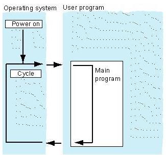
Organization Blocks and Program Structure:
Organization blocks (OBs) represent the interface between the operating system and the user program. Called by the operating system, they control cyclic and interrupt¬driven program execution, startup behavior of the PLC and error handling. You can program the organization blocks to determine CPU behavior.Organization Block PriorityOrganization blocks determine the sequence (start events) by which individual program sections are executed. An OB call can interrupt the execution of another OB. Which OB is allowed to interrupt another OB depends on its priority. Higher priority OBs can interrupt lower priority OBs. The background OB has the lowest priority.
Types of Interrupt and Priority Classes
Start events triggering an OB call are known as interrupts. The following table shows the types of interrupt in STEP 7 and the priority of the organization blocks assigned to them. Not all organization blocks listed and their priority classes are available in all S7 CPUs (see "S7-300 Programmable Controller, Hardware and Installation Manual" and "S7-400, M7-400 Programmable Controllers Module Specifications Reference Manual").
 Blocks for Different Connection Types:
Type of Interrupt
|
Organization Block
|
Priority Class
(Default)
|
See also
|
Main program scan
|
OB1
|
1
|
Organization Block for Cyclic Program Processing (OB1)
|
Time-of-day interrupts
|
OB10 to OB17
|
2
|
Time-of-Day Interrupt Organization Blocks (OB10 to OB17)
|
Time-delay interrupts
|
OB20
|
3
|
Time-Delay Interrupt Organization Blocks (OB20 to OB23)
|
OB21
|
4
|
||
OB22
|
5
|
||
OB23
|
6
|
||
Cyclic interrupts
|
OB30
|
7
|
Cyclic Interrupt Organization Blocks (OB30 to OB38)
|
OB31
|
8
|
||
OB32
|
9
|
||
OB33
|
10
|
||
OB34
|
11
|
||
OB35
|
12
|
||
OB36
|
13
|
||
OB37
|
14
|
||
OB38
|
15
|
||
Hardware interrupts
|
OB40
|
16
|
Hardware Interrupt Organization Blocks (OB40 to OB47)
|
OB41
|
17
|
||
OB42
|
18
|
||
OB43
|
19
|
||
OB44
|
20
|
||
OB45
|
21
|
||
OB46
|
22
|
||
OB47
|
23
|
||
DPV1 interrupts
|
OB 55
|
2
|
Programming DPV1 Devices
|
OB 56
|
2
|
||
OB 57
|
2
|
||
Multicomputing
interrupt
|
OB60 Multicomputing
|
25
|
Multicomputing - Synchronous Operation of Several CPUs
|
Synchronous cycle
interrupt
|
OB 61
|
25
|
Configuring Short and Equal-Length Process Reaction Times on
PROFIBUS-DP
|
OB 62
|
|||
OB 63
|
|||
OB 64
|
|||
Redundancy errors
|
OB70 I/O Redundancy Error (only in H systems)
|
25
|
"Error Handling Organization Blocks (OB70 to OB87 / OB121 to
OB122)"
|
OB72 CPU Redundancy Error (only in H systems)
|
28
|
||
Asynchronous errors
|
OB80 Time Error
|
25
|
Error Handling Organization Blocks (OB70 to OB87 / OB121 to
OB122)
|
OB81 Power Supply Error
|
(or 28 if the asynchronous
error OB exists in the start-up program)
|
||
OB82 Diagnostic Interrupt
|
|||
OB83 Insert/Remove Module Interrupt
|
|||
OB84 CPU Hardware Fault
|
|||
OB 85 Program Cycle Error
|
|||
OB86 Rack Failure
|
|||
OB87 Communication Error
|
|||
Background cycle
|
OB90
|
29 1)
|
Background Organization Block (OB90)
|
Startup
|
OB100 Restart
|
27
|
Startup Organization Blocks (OB100/OB101/OB102)
|
(Warm start)
|
27
|
||
OB101 Hot Restart
|
27
|
||
OB102 Cold Restart
|
|||
Synchronous errors
|
OB121 Programming Error
|
Priority of the OB
that caused the error
|
Error Handling Organization Blocks (OB70 to OB87 / OB121 to
OB122)
|
OB122 Access Error
|
|||
1) The priority
class 29 corresponds to priority 0.29. The background cycle has a lower
priority than the free cycle.
|
Changing the Priority:
Interrupts can be assigned parameters with STEP 7. With the parameter assignment you can for example, deselect interrupt OBs or priority classes in the parameter blocks: time ¬of ¬day interrupts, time¬delay interrupts, cyclic interrupts, and hardware interrupts.
The priority of organization blocks on S7-300 CPUs is fixed.
With S7-400 CPUs (and the CPU 318) you can change the priority of the following organization blocks with STEP 7:
•OB10 to OB47
•OB70 to OB72 (only H CPUs) and OB81 to OB87 in RUN mode.
The following priority classes are permitted:
•Priority classes 2 to 23 for OB10 to OB47
•Priority classes 2 to 28 for OB70 to OB72
•Priority classes 24 to 26 for OB81 to OB87; for CPUs as of approx. The middle of 2001 (Firmware Version 3.0) the ranges where extended: Priority classes 2 to 26 can be set for OB 81 to OB 84 as well as for OB 86 and OB 87.
You can assign the same priority to several OBs. OBs with the same priority are processed in the order in which their start events occur.
Error OBs started by synchronous errors are executed in the same priority class as the block being executed when the error occurred.
Local Data
When creating logic blocks (OBs, FCs, FBs), you can declare temporary local data. The local data area on the CPU is divided among the priority classes.
On S7-400, you can change the amount of local data per priority class in the "priority classes" parameter block using STEP 7.
Start Information of an OB
Every organization block has start information of 20 bytes of local data that the operating system supplies when an OB is started. The start information specifies the start event of the OB, the date and time of the OB start, errors that have occurred, and diagnostic events.
For example, OB40, a hardware interrupt OB, contains the address of the module that generated the interrupt in its start information.
Deselected Interrupt OBs
If you assign priority class 0 or assign less than 20 bytes of local data to a priority class, the corresponding interrupt OB is deselected. The handling of deselected interrupt OBs is restricted as follows:
•In RUN mode, they cannot be copied or linked into your user program.
•In STOP mode, they can be copied or linked into your user program, but when the CPU goes through a restart (warm start) they stop the startup and an entry is made in the diagnostic buffer.
By deselecting interrupt OBs that you do not require, you increase the amount of local data area available, and this can be used to save temporary data in other priority classes.
Cyclic Program Processing:
Cyclic program processing is the "normal" type of program execution on programmable logic controllers, meaning the operating system runs in a program loop (the cycle) and calls the
organization block OB1 once in every loop in the main program. The user program in OB1 is therefore executed cyclically.

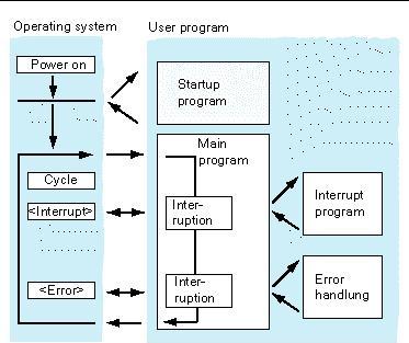
Event-Driven Program Processing:
Cyclic program processing can be interrupted by certain events (interrupts). If such an event occurs, the block currently being executed is interrupted at a command boundary and a different organization block that is assigned to the particular event is called. Once the organization block has been executed, the cyclic program is resumed at the point at which it was interrupted.

This means it is possible to process parts of the user program that do not have to be processed cyclically only when needed. The user program can be divided up into "subroutines" and distributed among different organization blocks. If the user program is to react to an important signal that occurs relatively seldom (for example, a limit value sensor for measuring the level in a tank reports that the maximum level has been reached), the subroutine that is to be processed when the signal is output can be located in an OB whose processing is event-driven.
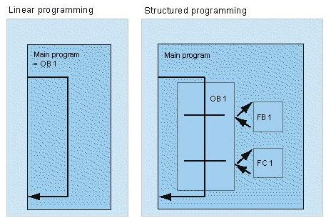
Linear Versus Structured Programming:
You can write your entire user program in OB1 (linear programming). This is only advisable with simple programs written for the S7-300 CPU and requiring little memory.
Complex automation tasks can be controlled more easily by dividing them into smaller tasks reflecting the technological functions of the process or that can be used more than once. These tasks are represented by corresponding program sections, known as the blocks (structured programming).

Blocks for Use with S7 Connections:
The system function blocks are integrated in the CPUs of the S7-400.
For S7-300, with newer CPUs and CPs, you can operate S7 communication actively (that is, as client) by means of the interface of the CP. The blocks (FBs) have the same number and designation as the SFBs of the S7-400; however, they must be called up cyclically in the user program of the S7-300-CPU. You can find the blocks in the SIMATIC_NET_CP library.
The CP must support the client function for S7 communication.
The CPU 317-2 PN/DP with PROFINET interface can also be configured as a client for S7 communication. In this case, the same blocks are used as in the case for the S7-300 with CP mentioned above. These blocks are also in the Standard Library (Communication Blocks/CPU_300). The client function is only available with the PROFINET interface.
SFB/FB/FC
|
Designation
|
Brief Description
|
SFB8/FB8
|
USEND
|
Uncoordinated data
exchange using a send and a receive SFB
|
SFB9/FB9
|
URCV
|
Max. length SFB 8/9:
440 bytes, split into 4x100 bytes.
|
Max. length FB 8/9:
160 bytes
|
||
SFB12/FB12
|
BSEND
|
Exchange blocks of
data of variable length between a send SFB and a receive SFB
|
SFB13/FB13
|
BRCV
|
Max. length SFB 12/13:
64 KB
|
Max. length FB 12/13:
32 KB
|
||
SFB14/FB14
|
GET
|
Read data from a
remote device
|
Max. length SFB 14:
400 bytes, split into 4x100 bytes
|
||
Max. length FB 14: 160
|
||
SFB15/FB15
|
PUT
|
Write data to a remote
device
|
Max. length SFB 15:
400 bytes, split into 4x100 bytes
|
||
Max. length FB 15: 160
|
||
SFB19
|
START
|
Execute a restart
(warm restart) on a remote device
|
SFB20
|
STOP
|
Switch a remote device
to STOP mode
|
SFB21
|
RESUME
|
Execute a hot restart
in a remote device
|
SFB22
|
STATUS
|
Specific query of the
status of a remote device
|
SFB23
|
USTATUS
|
Receive status
messages from remote devices
|
SFC62
|
CONTROL
|
Query the status of
the connection that belongs to an SFB instance
|
FC62
|
C_CNTRL
|
Query the status of a
connection (for S7 300 CPUs)
|
Blocks for Use with Point-to-Point Connections
For the PtP connection type you can use the SFBs BSEND, BRCV, GET, PUT, and STATUS (see above table).
You can also use the SFB PRINT:
SFB
|
Designation
|
Brief Description
|
SFB16
|
PRINT
|
Send data to a printer
|
Blocks for Use with FMS Connections
FB
|
Designation
|
Brief Description
|
|
FB 2
|
IDENTIFY
|
Identify the remote
device for the user
|
|
FB 3
|
READ
|
Read a variable from a
remote device
|
|
FB 4
|
REPORT
|
Report a variable to
the remote device
|
|
FB 5
|
STATUS
|
Provide the status of
a remote device on request from the user
|
|
FB 6
|
WRITE
|
Write variables to a
remote device
|
Blocks for Use with FDL, ISO¬on¬TCP, UDP and ISO Transport Connections as well as Email Connections
FC
|
Designation
|
Brief Description
|
FC 5
|
AG_SEND
|
Send data by means of
a configured connection to the communication partner (<= 240 bytes).
|
FC 6
|
AG_RECV
|
Receive data by means
of a configured connection from the communication partner (<= 240 bytes,
not email).
|
FC 50
|
AG_LSEND
|
Send data by means of
a configured connection to the communication partner.
|
FC 60
|
AG_LRECV
|
Receive data by means
of a configured connection from the communication partner (not email).
|
FC 7
|
AG_LOCK
|
Lock the external data
access by means of FETCH/WRITE (not for UDP, email).
|
FC 8
|
AG_UNLOCK
|
Unlock the external
data access by means of FETCH/WRITE (not for UDP, email).
|
Rules for Entering Ladder Logic Elements:
You will find a description of the Ladder Logic programming language representation in the "Ladder Logic for S7-300/400 - Programming Blocks" manual or in the Ladder Logic online help.
A Ladder network can consist of a number of elements in several branches. All elements and branches must be connected; the left power rail does not count as a connection (IEC 1131-3).
When programming in Ladder you must observe a number of guidelines. Error messages will inform you of any errors you make.
Closing a Ladder Network
Every Ladder network must be closed using a coil or a box. The following Ladder elements must not be used to close a network:
•Comparator boxes
•Coils for midline outputs _/(#)_/
•Coils for positive _/(P)_/ or negative _/(N)_/ edge evaluation
Positioning Boxes
The starting point of the branch for a box connection must always be the left power rail. Logic operations or other boxes can be present in the branch before the box.
Positioning Coils
Coils are positioned automatically at the right edge of the network where they form the end of a branch.
Exceptions: Coils for midline outputs _/(#)_/ and positive _/(P)_/ or negative _/(N)_/ edge evaluation cannot be placed either to the extreme left or the extreme right in a branch. Neither are they permitted in parallel branches.
Some coils require a Boolean logic operation and some coils must not have a Boolean logic operation.
- Coils which require Boolean logic:
Output _/( ), set output _/(S), reset output _/(R)
Midline output _/(#)_/, positive edge _/(P)_/, negative edge _/(N)_/
All counter and timer coils
Jump if Not _/(JMPN)
Master Control Relay On _/(MCR<)
Save RLO into BR Memory _/(SAVE)
Return _/(RET)
- Coils which do not permit Boolean logic:
Master Control Relay Activate _/(MCRA)
Master Control Relay Deactivate _/(MCRD)
Open Data Block _/(OPN)
Master Control Relay Off _/(MCR>)
All other coils can either have Boolean logic operations or not.
The following coils must not be used as parallel outputs:
- Jump if Not _/(JMPN)
- Jump _/(JMP)
- Call from Coil _/(CALL)
- Return _/(RET)
Enable Input/Enable Output
The enable input "EN" and enable output "ENO" of boxes can be connected but this is not obligatory.
Removing and Overwriting
If a branch consists of only one element, the whole branch is removed when the element is deleted.
When a box is deleted, all branches which are connected to the Boolean inputs of the box are also removed with the exception of the main branch.
The overwrite mode can be used to simply overwrite elements of the same type.
Parallel Branches
- Draw OR branches from left to right.
- Parallel branches are opened downwards and closed upwards.
- A parallel branch is always opened after the selected Ladder element.
- A parallel branch is always closed after the selected Ladder element.
- To delete a parallel branch, delete all the elements in the branch. When the last element in the branch is deleted, the branch is removed automatically.
Constants
Binary links cannot be assigned constants (i.e. TRUE or FALSE). Instead, use addresses of the data type BOOL.
Creating a Closed Branch in Ladder Networks:
To create a closed branch, proceed as follows:
1.Select the element in front of which you want to open a parallel branch.
2.Open the parallel branch with F8.
3.Insert the Ladder element.
4.Close the branch with F9.
The following example shows how you create a branch using only function keys or toolbar buttons.
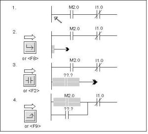

When you close parallel branches, any necessary empty elements are added. If necessary, the branches are arranged so that they do not cross over. If you close the branch directly from the parallel branch, the branch is closed following the next possible Ladder element.
Language Elements of S7-PDIAG:
Using language elements, you can program your specific general monitoring logic.
It is important that you only use language elements which belong to the programming languages of S7-PDIAG when entering monitoring logic, and that you arrange these language elements in the correct syntax.
Any syntax errors in the monitoring logic are reported when you attempt to save your changes. All characters which are valid as identifiers for addresses or timers in STEP 7 are permitted.
S7-PDIAG supports the following programming language elements:
AND, ONDT, EN, EP, NOT, OR, SRT, XOR, Separators, Brackets, Addresses, Timers, Set and Reset Assignments
Parameter Types:
In addition to elementary and complex data types, you can also define parameter types for formal parameters that are transferred between blocks. STEP 7 recognizes the following parameter types:
- TIMER or COUNTER: this specifies a particular timer or particular counter that will be used when the block is executed. If you supply a value to a formal parameter of the TIMER or COUNTER parameter type, the corresponding actual parameter must be a timer or a counter, in other words, you enter "T" or "C" followed by a positive integer.
- BLOCK: specifies a particular block to be used as an input or output. The declaration of the parameter determines the block type to be used (FB, FC, DB etc.). If you supply values to a formal parameter of the BLOCK parameter type, specify a block address as the actual parameter. Example: "FC101" (when using absolute addressing) or "Valve" (with symbolic addressing).
- POINTER: references the address of a variable. A pointer contains an address instead of a value. When you supply a value to a formal parameter of the parameter type POINTER, you specify an address as the actual parameter. In STEP 7, you can specify a pointer in the pointer format or simply as an address (for example, M 50.0). Example of a pointer format for addressing the data beginning at M 50.0: P#M50.0
- ANY: this is used when the data type of the actual parameter is unknown or when any data type can be used. For more information about the ANY parameter type, refer to the sections "Format of the Parameter Type ANY" and "Using the Parameter Type ANY".
Parameter
|
Capacity
|
Description
|
TIMER
|
2 bytes
|
Indicates a timer to
be used by the program in the called logic block.
|
Format: T1
|
||
COUNTER
|
2 bytes
|
Indicates a counter to
be used by the program in the called logic block.
|
Format: C10
|
||
BLOCK_FB
|
2 bytes
|
Indicates a block to
be used by the program in the called logic block.
|
BLOCK_FC
|
Format: FC101
|
|
BLOCK_DB
|
DB42
|
|
BLOCK_SDB
|
||
POINTER
|
6 bytes
|
Identifies the
address.
|
Format: P#M50.0
|
||
ANY
|
10 Bytes
|
Is used when the data
type of the current parameter is unknown.
|
Format:
|
||
P#M50.0 BYTE 10 ANY format for data types
|
||
P#M100.0 WORD 5
|
||
L#1COUNTER 10 ANY format for parameter types
|
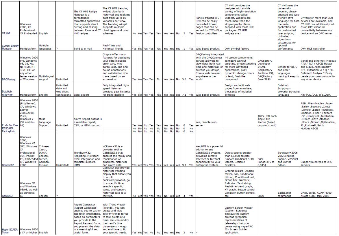
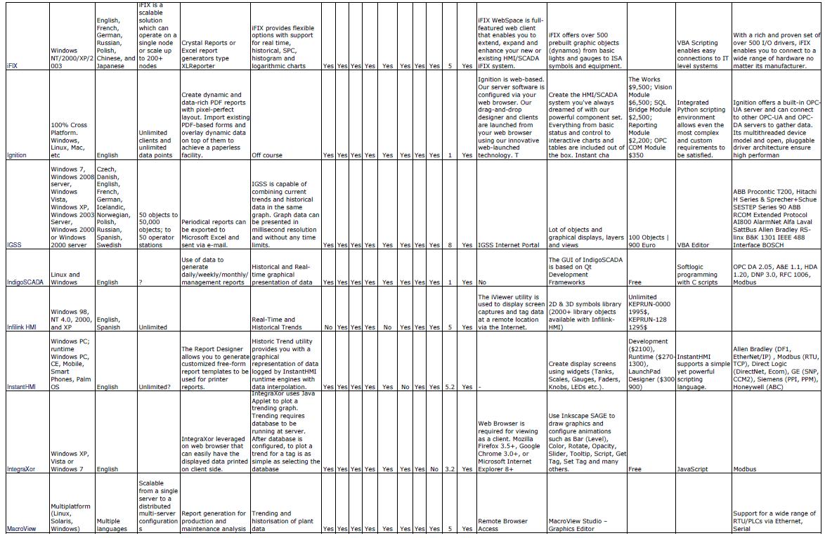
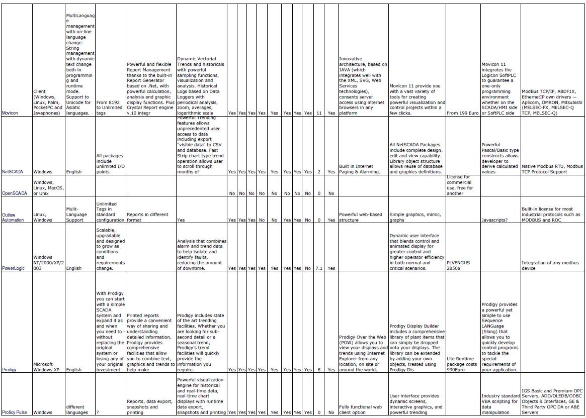
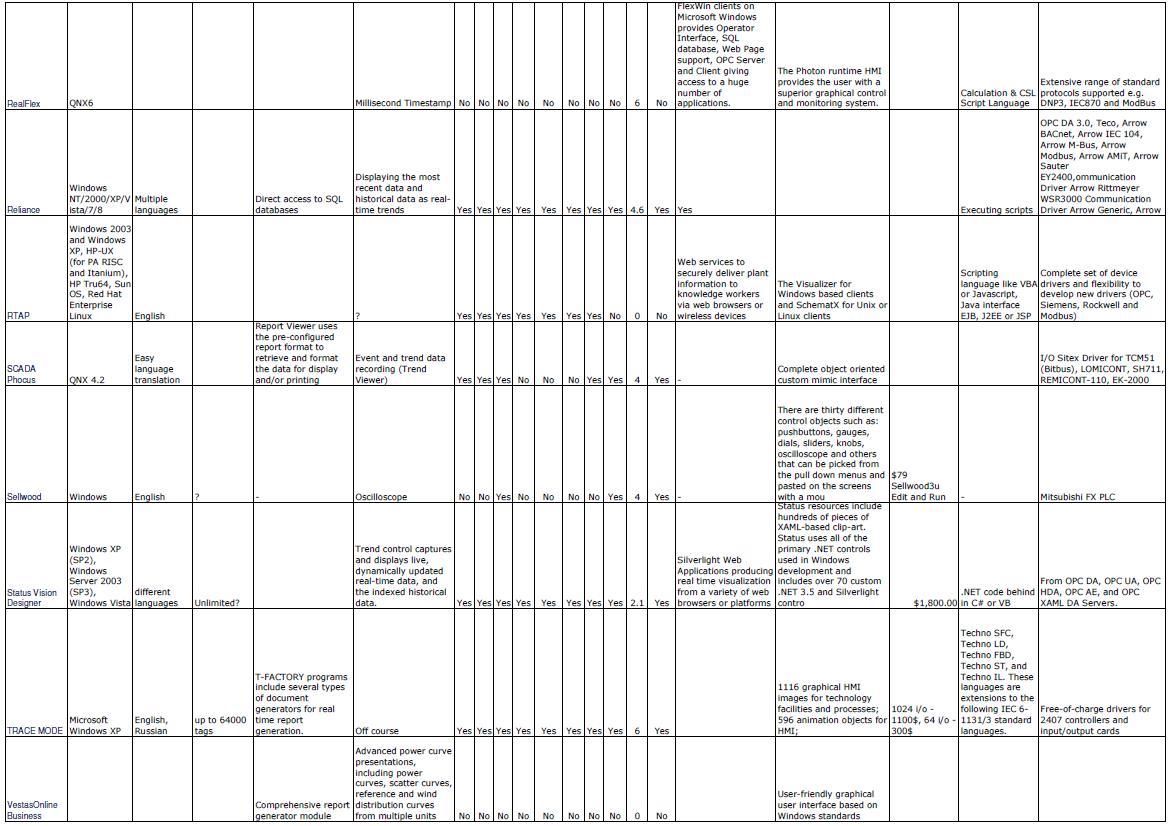
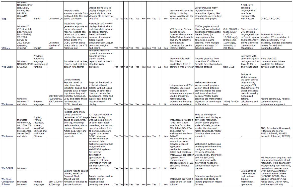
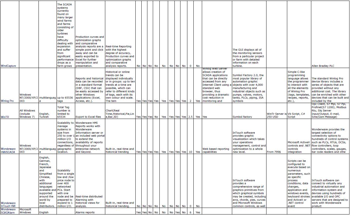
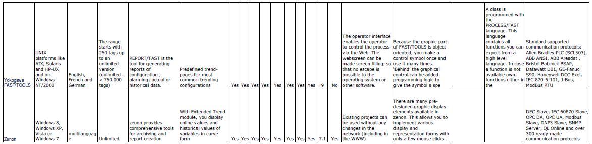
4. Supervisory Control And Data Acquisition (SCADA).
- SCADA Packages
- Role of SCADA in industrial automation:
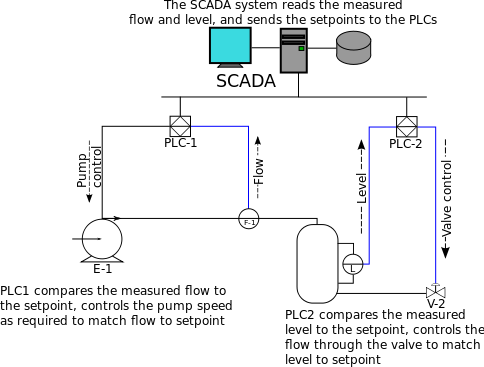
SCADA (supervisory control and data acquisition) is a type of industrial control system (ICS). Industrial control systems are computer controlled systems that monitor and control industrial processes that exist in the physical world. SCADA systems historically distinguish themselves from other ICS systems by being large scale processes that can include multiple sites, and large distances.[1] These processes include industrial, infrastructure, and facility-based processes, as described below:
- Industrial processes include those of manufacturing, production, power generation, fabrication, and refining, and may run in continuous, batch, repetitive, or discrete modes.
- Infrastructure processes may be public or private, and include water treatment and distribution, wastewater collection and treatment, oil and gas pipelines, electrical power transmission and distribution, wind farms, civil defense siren systems, and large communication systems.
- Facility processes occur both in public facilities and private ones, including buildings, airports, ships, and space stations. They monitor and control heating, ventilation, and air conditioning systems (HVAC), access, and energy consumption.
Common system components:
A SCADA system usually consists of the following subsystems:
- A human–machine interface or HMI is the apparatus or device which presents processed data to a human operator, and through this, the human operator monitors and controls the process.
- SCADA is used as a safety tool as in lock-out tag-out
- A supervisory (computer) system, gathering (acquiring) data on the process and sending commands (control) to the process.
- Remote terminal units (RTUs) connecting to sensors in the process, converting sensor signals to digital data and sending digital data to the supervisory system.
- Programmable logic controller (PLCs) used as field devices because they are more economical, versatile, flexible, and configurable than special-purpose RTUs.
- Communication infrastructure connecting the supervisory system to the remote terminal units.
- Various process and analytical instrumentation
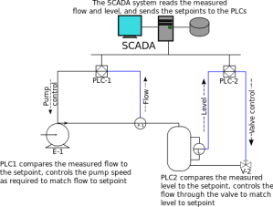
Systems concepts:
The term SCADA usually refers to centralized systems which monitor and control entire sites, or complexes of systems spread out over large areas (anything from an industrial plant to a nation). Most control actions are performed automatically by RTUs or by PLCs. Host control functions are usually restricted to basic overriding or supervisory level intervention. For example, a PLC may control the flow of cooling water through part of an industrial process, but the SCADA system may allow operators to change the set points for the flow, and enable alarm conditions, such as loss of flow and high temperature, to be displayed and recorded. The feedback control loop passes through the RTU or PLC, while the SCADA system monitors the overall performance of the loop.
Data acquisition begins at the RTU or PLC level and includes meter readings and equipment status reports that are communicated to SCADA as required. Data is then compiled and formatted in such a way that a control room operator using the HMI can make supervisory decisions to adjust or override normal RTU (PLC) controls. Data may also be fed to an Historian, often built on a commodity Database Management System, to allow trending and other analytical auditing.
SCADA systems typically implement a distributed database, commonly referred to as a tag database, which contains data elements called tags or points. A point represents a single input or output value monitored or controlled by the system. Points can be either "hard" or "soft". A hard point represents an actual input or output within the system, while a soft point results from logic and math operations applied to other points. (Most implementations conceptually remove the distinction by making every property a "soft" point expression, which may, in the simplest case, equal a single hard point.) Points are normally stored as value-timestamp pairs: a value, and the timestamp when it was recorded or calculated. A series of value-timestamp pairs gives the history of that point. It is also common to store additional metadata with tags, such as the path to a field device or PLC register, design time comments, and alarm information.
SCADA systems are significantly important systems used in national infrastructures such as electric grids, water supplies and pipelines. However, SCADA systems may have security vulnerabilities, so the systems should be evaluated to identify risks and solutions implemented to mitigate those risks.
For the below Topic kindly go through the following links & Videos for better understanding of SCADA:
- SCADA system configuration, RTU, communication protocols.
- Script programming.
- Real time and historical trend.
- Configuring Alarms.
- Real time project development with PLC interfacing.
- Communication with other software.
- Recipe management.
- Accessing different security levels.
- Report generation of current plant.
Part-1 for WINCC
Part-2 for WINCC
INTRODUCTION TO SCADA WinCC:
A SCADA system is a program that will allow monitoring, acquisition and processing of data that come from a process.
Click this link to know about WINCC process control which contains:(Working with Projects, Working with Projects, Opening WinCC Explorer, Closing WinCC Explorer, The WinCC Explorer, Project Types, Creating and Editing Projects, Preparation to Create a Project, WinCC Project with Basic Process Control, How to Create a Project, How to Specify the Computer Properties, How to support multiple picture windows, Setting Time in WinCC, Online Configuration, Loading Online Changes, Determining the Global Design, Making Settings for Runtime, Activating Project, Copying and Duplicating Projects, Appendix, Working with Tags, Creating Process Pictures, Process Picture Dynamics, Setting up a Message System, Archiving Process Values, Documentation of Configuration and Runtime Data, Creating Page Layouts, Creating Line Layouts, Setting Up Multilingual Projects, Structure of the User Administration, Integration of WinCC in SIMATIC Manager, WinCC/Options for Process Control, Modbus TCPIP)
WinCC/Options for Process Control
1. Creating a new project:
To create a new project will follow the following steps:
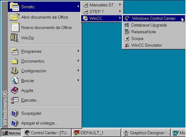
1. Open SCADA from the "Start" menu.
2. Then drop down the "File" menu and select "New", so a screen which will give the project a name and click the "Create" button.3. Once this is done will the project created with the following structure:
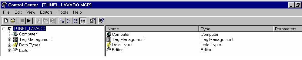
Let's look at each element of the tree:
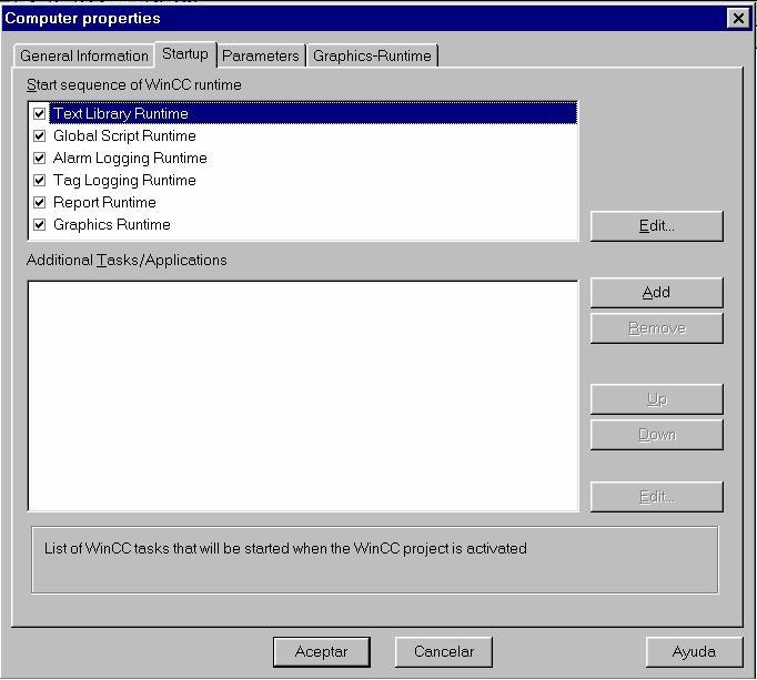
Computer: We will select applications or tasks that we want
our project started when activated. To do this we will:
1. Select "Computer" and left mouse button we double. Click on the icon that appears in the right window.
2. Then choose the tab "Startup" and we enable applications we want to boot with our project.
Press the button"OK" once selected as desired.
Tag Management: This element will define the internal variables SCADA, external variables and communication drivers and connection with the automaton.
Data Types: When expanded appear all possible types of data so that when you select one displayed in the right window of the project variables whose format is selected. Editor: When expanded appear various types of editors available.
To open any of the editors select enough with the right mouse button and choose "Open".
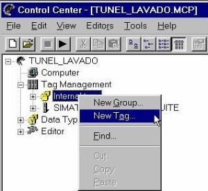
2. Creating an internal variable:
They are located in memory variables SCADA. For its creation we will:
We expand the branch "Tag Management" and select "Internal tags" with the right mouse button.
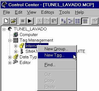
Select "New" so that a window will appearconfigure the variable.
Finally will press "OK" to save the configuration.
3. Creating an external variable:
An external variable is one that is directly related to the process. Before creating external variables need to configure communication drivers between the PLC and SCADA.
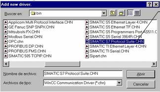
- Select "Tag Management" with the right mouse button and choose "Add New Driver ". You will see the available drivers and select the desired one.
Then press the button "Open", so that the driver will appear in the hierarchical tree.
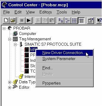
- Then expand the driver that appears in the tree and select the connection type in
our case MPI, with the right mouse button and choose "New Driver Connection ".
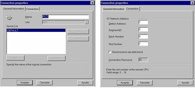
- Finally enter the name of the connection (PLC1) and parameters.
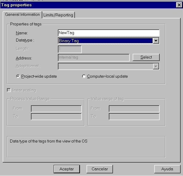
To create an external variable:
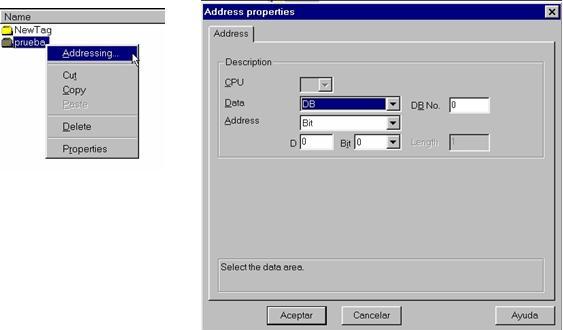
• Select the connection PLC1 with right mouse button and choose "New tag ". A window where you choose the name and data type, finally pressing "OK".
• Then select with the right mouse button the variable created appears in the right window and choose the command "Addresing" (Fig.1). In the window that appears choose the type of data and corresponding address in the PLC.
Finally press the button "OK".
4. Creating images:
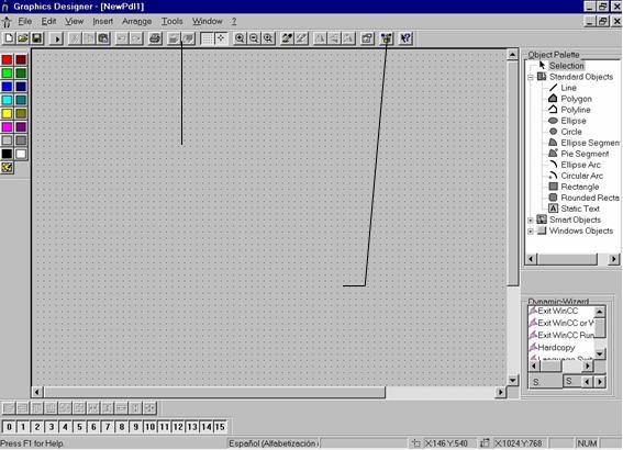
For imaging we use the graphical editor, Graphic Designer ", where we define our animations which will be controlled by internal and external variables SCADA.
To create an image you will:
- With the right mouse button will press the editor "Graphic Designer" and select "New Picture".
- In the right window shows "NewPdl0.Pdl" so that it select with the right mouse button and choose the command "Rename" to give it the name you want.
- To open the image double click it will appear as follows:
5. Types animations:
We define a number of basic animations:
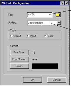
5.1 Setting a field input / output. Such an input / output can be used to represent the value of some variable. To do this we will:
• In the graphical editor select the "I / O field" group "Smart Object "and then drag it to the desired position where we.
click the mouse, appear a window where you configure this field.
Finally press the button "OK"
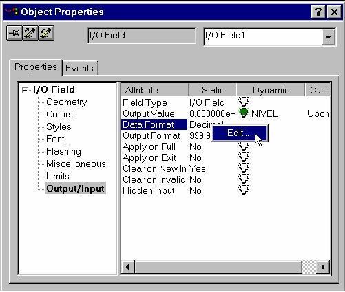
Once done select the object with the right mouse button and choose "Properties". Select the property "Output / Input" and in the window right select the attribute "Data Format" to choose the format variable representation.
5.2
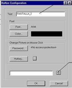
Changing from one screen to another by button.
In the graphical editor select the "Button" in the "Windows Object "and drag it to the desired position. Once there we click the mouse appear a window like the one below where we set the button.
Then click the button (1) of so that a window will appear choose the screen that jump.
Finally press the button "OK" to validate the configuration.
5.3 Setting a button to exit the application.
• In the graphical editor select the "Button" in the "Windows Object "and drag it to the desired position. Once done select it with the left mouse button.
Then double click on the "Exit WinCC Runtime" that appears in the "Dynamic Wizard". A wizard so that on the first screen press "Next" in the second choose "Left mouse key "and click" Next "and the last click" Finish ". This way when you press the button with the left mouse button, we will leave the application.
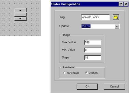
5.4 Controlling the value of a variable via pushbuttons.
- In the graphical editor select the "Slider Object" group "Windows Object". Then place the cursor in the desired position and click the left mouse button, appear a window where you configure the object.(Fig.1)
- Finally press the button "OK" to confirm the settings
Figure 2 shows the shaped element.
1: Variable whose value will force. 2: Update time.
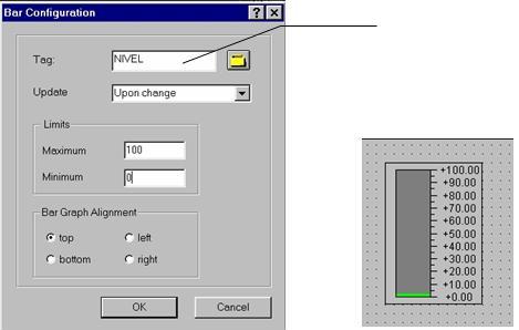
5.5 Animation of a variable in a bar graph.
• In the graphical editor select the "Bar" in the "Smart Object". A
Then place the cursor in the desired position and press the button left mouse button, a window popping configure the item.
• After configuring the item, press the button "OK" to give the element as shown in Figure 2
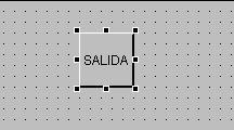
5.6 Make an object visible or not depending on the value of a variable bool
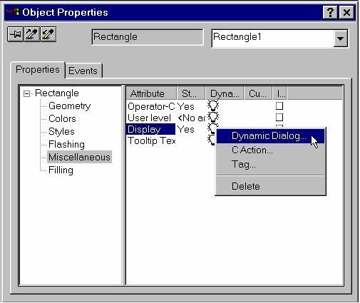 Then select the command "Dynamic Dialog" for configure the item.
- Select the object with the right mouse button and choose the command "Properties". Then select the property "Miscellaneous" and chose the right mouse button column "Dynamic" attribute "Display".
- A window like the one below where we set the element.
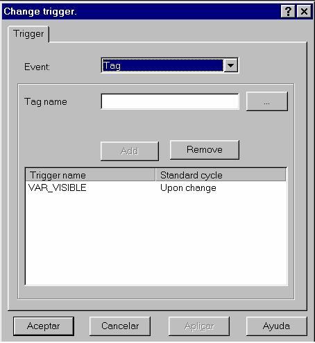
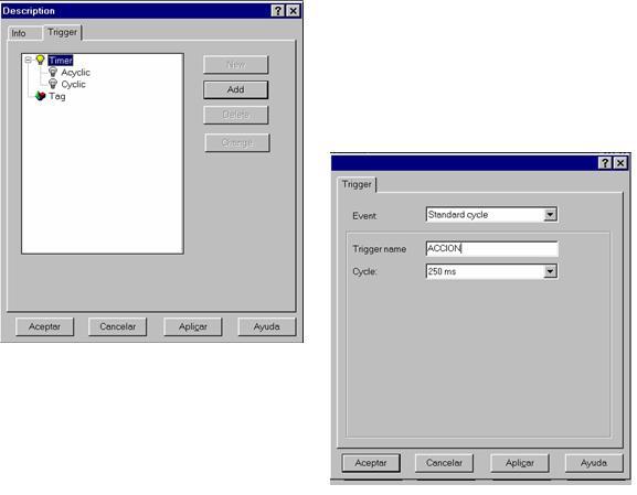
- Then press the button to set the trigger. Appears A window like the one below where you configure.
The firing cycle is chosen selecting the column "Standard cycle "with the right mouse. Once set will press the "OK", so return to the previous window and press the button "Apply".
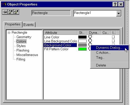
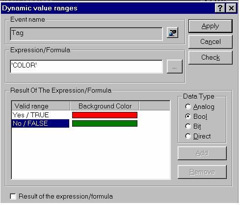
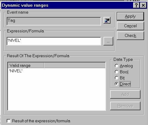
5.7 Change of color of an object. In this animation we will see how an object changes color depending on the value of a variable bool.
- Select the object with the right mouse button and choose the command "Properties". Then select the property "Colors" and chose to right-click the column Color ". "Dynamic" attribute "Background
Then choose the command "Dynamic Dialog" so that appear A window configure the item.
In the same way that the previous animation select the variable, the data type and the range of operation. For this choose the column "Valid range "with the right mouse and select the range. In like manner choose the column "Background Color" and choose the desired colors.
- Finally configure the trigger as described in the previous animation and finally press the button "Apply" to validate the configuration.
5.8 Changes in size of an object.
This animation shows how we can change the height and width of an object. See for height variation since the width variation will be identically.
- Select the object with the right mouse button, choose the command "Properties" and select the property "Geometry".
- Then select with the right mouse button on the column "Dynamic" attribute "Height", appearing as a window where where we will setup earlier. In this case when we select the data type choose "Direct" so that the selected attribute take the value of the associated variable which will modify its value in an "Action" planned for us. In later sections we will see how programming these "Actions" in the editor "Global Script".
- Finally configure the trigger in the same way that in the previous cases and press the button "Apply" to save the settings.
5.9 Movements of objects.
In this section we will endow an object moving in the X direction,knowing that we give it the same way as Y. motion
• select the object with the right mouse button, choose the command "Properties" and select the property "Geometry".
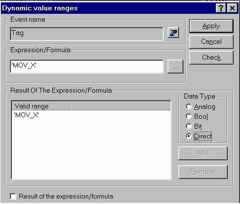
• Then select the column "Dynamic" attribute "Position X" and choose the command "Dynamic Dialog", so that a window where we set the object. In this window, choose the variable associated with the attribute and the type of data as in the previous case will choose a data type "Direct" so that this attribute will vary as it goes by the value of the variable within the "Action" that we have programmed in the publisher "Global Script ". (Paragraphs later)
• Finally configure the trigger as described in section 5.7 and press the button "Apply" to confirm the settings.
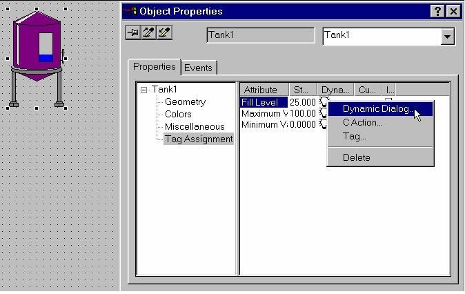
5.10 Evolution of the level in a tank.
• Select the deposit library available in the graphical editor. To so, click the button on the toolbar and expanded folder "Smart Object" select the folder where "Tank", choosing the desired tank being dragged with the mouse to the desired position.
• Then select the tank with the right mouse button, choose the command "Properties" and select the property "Tag Assigment ".
• Then select the column "Dynamic" attribute "Fill level" with the right mouse button, choose "Dynamic Dialog" and a window, as in the previous cases, where we set the object. As in the previous case the data type choose "Direct" so that the variable reservoir level associated evolve into an "Action" scheduled in the editor "Global Script".
The configuration window is:
Then press the button 1 to set the trigger.
Finally, press the button "Apply" to validate the configuration.
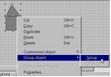
Note: You can make animations of objects which consist of grouping of several objects. To group objects together we will:
• With the left mouse button pressed objects locked in a room and then press the right mouse button.
• Then select the command "Group".
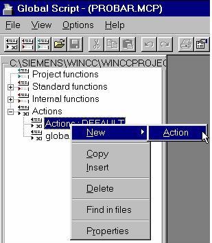
6. Scheduling an "Action":
An "Action" is a C function that can only be used in the project that has been created and will be provided as a trigger that we have scheduled. To schedule an "Action" will:
• With the right mouse button select the editor "Global Script" and opened.
• expanded then "Actions" and select with the right mouse button mouse "Actions-New-Action".
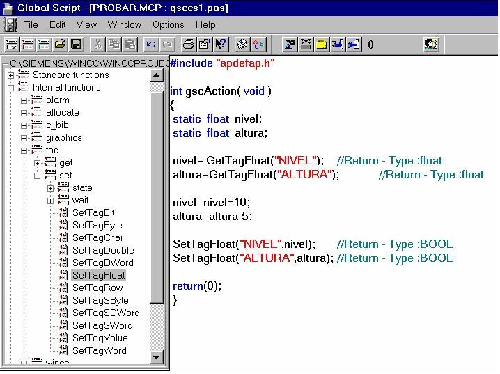
On the right will open a window where will schedule our "Action".
In the "Action" we believe we can use functions already created, "Standard function" and "Internal function", and even we can program our own functions by selecting "Project function ".
The most used functions are internal functions "Get" and "Set". To function "Get" will be assigned to a variable of the "Action" the value of a SCADA variable and using the "Set" will be assigned to a variable of SCADA the value of a variable in the "Action". For insertion into the "Action" just double clicking on them in the left window and then assign the appropriate parameters.
- Then we will compile the "Action" created by pressing that appears in the toolbar.
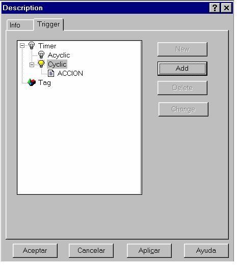
- Now configure the trigger of the "Action". For this press the button that appears in the toolbar and select the tab trigger.
Then select "Cyclic" and click the "Add" so A window in which select the trigger and once press the button configured "OK"
- After configuring the trigger, back to window 1 where will press "OK" to confirm the settings.
• Finally select "Save" the menu "File" and then will leave the editor "Global Script".
7. Creating charts and tables:
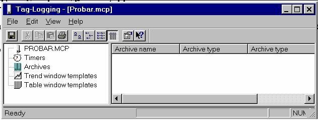
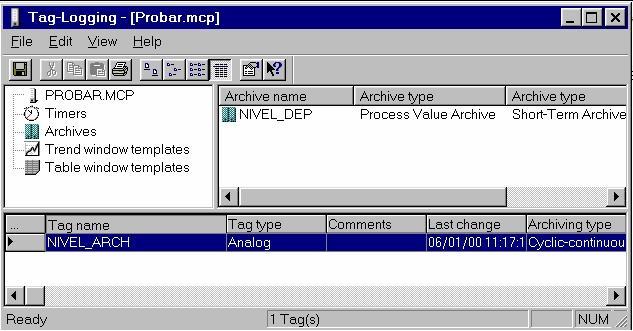
In this section we will take care of purchasing process and represent data in tables and graphs. The first thing you do is open the editor "Tag Logging":
7.1 Creating a data file:
To create this file we will use the wizard "Archive Wizard":
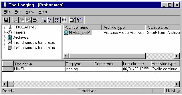
1. Select "Archives" with the right mouse button and choose "Archive Wizard":
1st screen: Click on "Next".
2nd screen: Insert the name of the data file, eg "NIVEL_DEP" and the file type, eg "Process Value Archive", and click "Next".
3rd screen: Press "Select" and choose the process variable that we will represent and click "Finish".
2. Then select the process variable in the lower window with the right mouse button and choose "Properties". A window in which we introduce "NIVEL_ARCH" as variable name archived. Then select the tab cycle properties:
Acquisition: 500 ms.
Archiving: 1 * 500 ms
Press the button "OK"."Parameter" and introduce the Effect is that the process variable "LEVEL" is acquired each 500 ms and stored as a variable called "NIVEL_ARCH".
3. Finally deploy the "File" menu and select "Save" to save the settings.
7.2 Creating a graph:
For graphical representation of the values of the variable use archived.
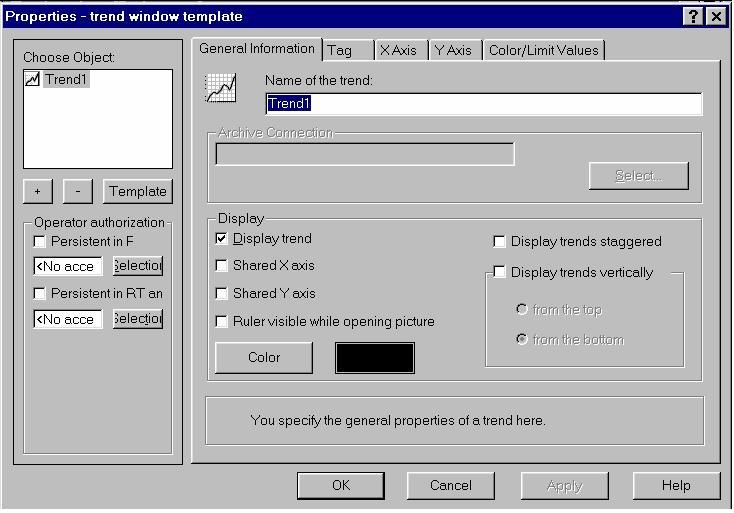
- Select with the right mouse button "Trend window templates" and choose "New", appearing a window as shown:
- select the "Template" and enter "EVOL_NIVEL" as the template name and click "OK".
- In the tab "General Information" enter "NIVEL_DEP" as the trend name (Name of the trend) we are going to portray.
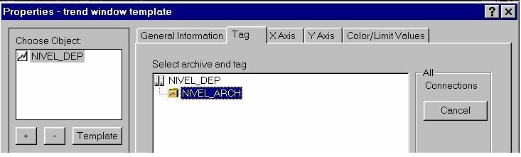
- In the tab "Tag" will double click on the file name "NIVEL_DEP" and select the variable that we will represent archived.
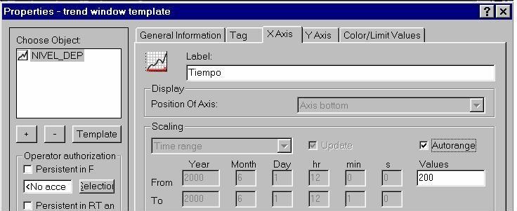
- In the tab "X Axis" enter the name of the X axis "Time" and will qualify the box "Auto range" introducing 200 as the value to climb.
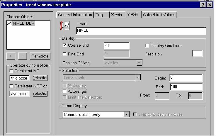
- In the tab "Y Axis" enter the name of the Y axis, "Level", will qualify the box "Coarse grid" with a value of 20, we will disable the box "Auto range" and introduce "0" initial value "100" as final value and finally select "Connect dots linearly" in the box "Trend Display".
- Finally press the button "OK" to save the settings.
7.3 Inserting a graph in an image:
- First open the graphical editor, and then the image where you want to insert the chart.
- Select the object "Application Window" in the "Smart Object" that is located in the "Object Palette".
- After selecting move the cursor to the desired position image and press the left mouse button popping a window called "Windows Contents" which select "Tag Logging", pressing then "OK".
- A window called "Template" that will select the template "EVOL_NIVEL" we're going to represent, and press "OK".
- Finally we will give to the window, which appears with the name we have given to the template, the desired size and will save the configuration.
7.4 Creating a table of values:
In this section we will create a table of values of a process variable.
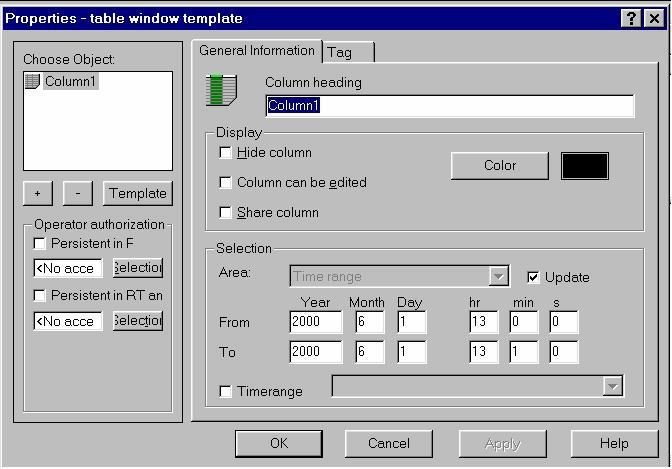
- Select with the right mouse button "Table window templates" in the editor "Tag Logging" and choose "New", appearing as a window shown:
- Select the "Template" and enter "level_value" as the template name, then pressing "OK".
- In the tab "General Information" introduce "LEVEL" as the table header.
- In the tab "Tag" will double click on the file name, "NIVEL_DEP" and select the variable "NIVEL_ARCH". Then press the button "OK".
- Finally deploy the "File" menu and select "Save" to save the configuration.
7.5 Insert a table into an image:
- First open the graphical editor, and then the image where want to insert the table.
- Select the object "Application Window" in the "Smart Object" that is located in the "Object Palette".
- After selecting move the cursor to the desired position image and press the left mouse button popping a window called "Windows Contents" which select "Tag Logging", pressing then "OK".
- A window called "Template" that will select the template "level_value" we're going to represent, and press "OK".
- Finally we will give to the window, which appears with the name we have given to the template, the desired size and will save the configuration.
8. Message Settings:
This section is intended to show how messages are configured and texts associated with them.
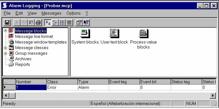
- First open the message editor called "Alarm Logging" popping up a screen as shown:
- Then pluck the message wizard displaying the "File" menu and select the command "Start Message Wizard":
1st screen: Click on "Next".
2nd screen: select Date, Time, Number system block and Msg, Location Error in user text blocks and click "Next".
3rd screen: Press "Next" preset leaving the box.
4th screen: Select "Without Bars" and click "Next".
5th screen: Press "Next" preset leaving the box.
6th screen: Select "Short-Term Archive for 250 Message" and press "Next".
7th screen: Click on "Next".
8th screen: Press "Finish".
- If we add other blocks to our message that have not been added by the wizard, do the following:
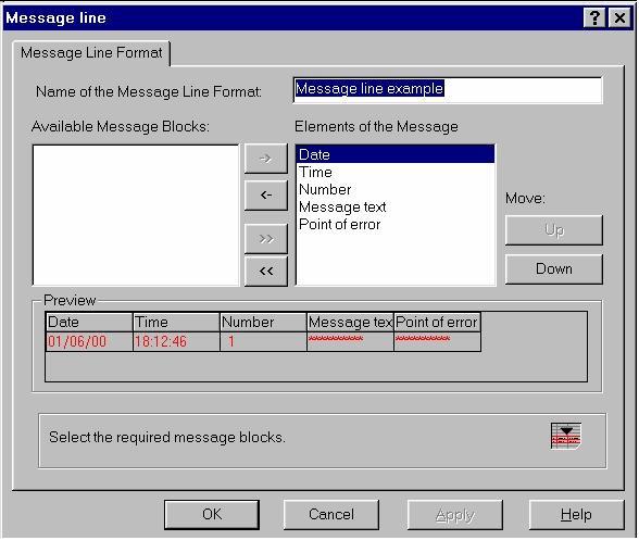
1. Select the line "Message line format" in the left window editor.
2. With the right mouse button select "Message Line Example" link on the right of the editor window and select "Properties".
3. A window in which we can add the blocks "Message Text" and "Point of Error" message to our line.
Once done this, press the button "OK".
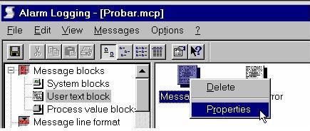
- If we change the number of characters associated with the block "Message text ", we will:
1. We expanded the line "Message Blocks" and select the line "User Text Block". Then select with the right mouse button "Message text" on the right of the editor window.
Select the command "Properties" so that a window where we can enter 30 as the number of characters associated with the block and press "OK". To say that in the same way we can change the number of characters associated with the block "Point of Error".
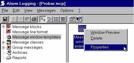
- If we want to change the message window will:
1. Select the line "Message window templates" and then with the right mouse button select "Message Window Example" on the right of the editor window.
2. Select the command "Properties" so that it will open a window with several tabs:
- General Information: We will enter the name of the window, the title of the window and choose "Short-Term Archive Window" as a kind of window.
- Parameters: lockers will qualify "Line Title" and "Column Title".
- Status Bar: will qualify the boxes "Show Status Bar", "Date", "Time" and choose "Bottom" as alignment.
- Toolbar: will qualify all key functions except "City Call" will qualify "Show Toolbar" and choose "Top" as alignment.
3. Finally press the button "OK".
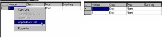
- To set the text of a message we will:
1. Select with the right mouse button on the column "Number" of the lower window and choose "Append New Line". In this manner add a new row and so many rows as we have messages.
2. In Row 1 will configure the first message. Double clicking on the column "Event tag" select the variable that will cause me message. If this variable is a 16 bit and the third bit is the bit that when going from 0-1 I will produce the message, column Event bit" will place February 1. (16 2 1 0). If this variable is bit, in the "Event bit" was to be nothing.
3. Here we introduce in the "Messsage text" the message you want to appear, such as "empty tank". Similarly we can enter messages in the "Point of Error".
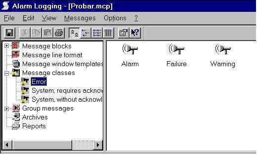
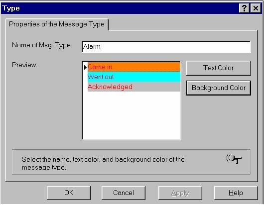
- Then we will endow our messages of a color depending on whether it is a valid message, a different color if the message is no longer valid and another color if recognized message. To do this we will:
1. We expanded "Message Classes" and select the line "Error".
2. Then select with the right mouse button icon "Alarm" appears in the right window and choose "Properties".
3. A window appears in which you configure the color of the text and the background color simply by selecting the character of the message and pressing the "Text Color" and "Background Color" to choose the colors.
Finally will press "OK" to validate configuration.
- Having done all this, we will display the "File" menu and select "Save" to save the settings.
8.1 Insert a message window in an image.
- First open the graphical editor, and then the image where want to insert the message window.
- Select the object "Application Window" in the "Smart Object" that is located in the "Object Palette".
- After selecting move the cursor to the desired position image and press the left mouse button popping a window called "Windows Contents" which select "Alarm Logging", pressing then "OK".
- A window called "Template" that will select the template "NIVEL_DEPOSITO" we're going to represent, and press "OK".
- Finally we will give to the window, which appears with the name we have given to the template, the desired size and will save the configuration.
9. Start an application:
To start the application and see how the process evolves we have two possibilities:
1. Acting from the "Control Center" enabling or disabling the icons situation in the toolbar.
2. Acting from the "Graphic Designer" activating the icon located in the toolbar.
10. Using SCADA simulator:
WINCC is provided with a simulator called WinCC Simulator with which we check whether our application works fine without have a physical automaton we generate external signals. In this case no work with external variables but with internal variables which are associate a certain manner to simulate evolution behavior Real.
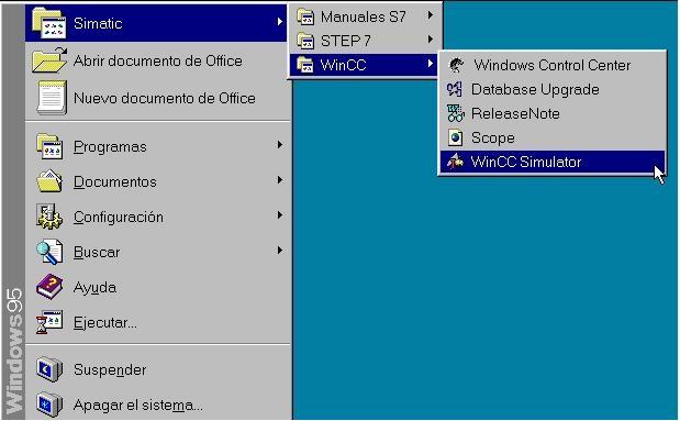
1. First open the simulator as shown in
figure:
Note that the image that we encourage must be enabled before setting the simulator.
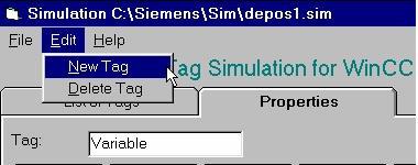
2. After opening the simulator we will define the variables that we want to simulate. To do this select "Edit" from the menu bar and choose "New Tag".
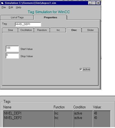
3. In the tab "Properties" enter the name of the desired tag and Then choose the mode of evolution of the variable. We see that we can choose between different types of development which we will parameterized:
- Sine: In this type of evolution specify the parameters of a sinusoidal function such as the amplitude, which specify the range of values, the period of the function and offset.
- Evolution oscillatory: We introduce the parameter "Setpoint" where will indicate the value after the event transient, the parameter "Overshoot" which indicate As can be away from the setpoint values, the oscillation period and the parameter "Damping".
- Random Evolution: Here specify the range of values that our variable.
- Increasing linear evolution: We specify the starting value and the value end.
- Decreasing linear evolution: In the same way specify the start and end values.
- Evolution with a slider: We specify the start and end value.
We will choose a linear evolution for variable NIVEL_DEP1 decreasing and increasing linear trends for the variable NIVEL_DEP2.
4. Then the box will qualify "active".
5. Having done all this, we go to the tab "List of Tags' and see as the variables we selected for simulation are varying their values. (Fig.2)
5 . Introduction to DCS
- Architecture of DCS
- Yokogawa Centum CS 3000
- Comparison of PLC with DCS
- Programming languages for DCS
- Different types of cards and their functions
6 . Control Panel Designing
- Different types of panels.
- Basic components to be installed in a panel.
- Wiring details of panel.
- Specification and physical dimension of components.
- Earthing and Cabling of Panels- standard procedures.
- P&I diagram
No comments:
Post a Comment